Hello everyone, I encountered an unexpected stop when using SOS to calculate the second-order susceptibility, like this
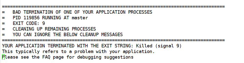
After checking the log file, I found that this happened in the fourth dataset, corresponding to the computation of the ddk matrix elements. Is this a problem caused by insufficient memory?
My physical memory is 128G, and the swap partition is 20G. The calculation system contains eight atoms, the K-point mesh is 9 9 9 (low, only for test), and it can run normally when running the same calculation file before and there is no similar error.
Hope someone can help me solve this problem, thank you very much.
Hello Lamed, thank you for your question! Would you please send us your input file, your log file and any stderr file if relevent. That could help us solve your issue.
Thank you very much for your reply. This is my related file. Please help me to check it. I don’t know if the parallel parameter autoparal=1 can be used when deriving the wave function. Because I compared the calculations before and after and found that this is the biggest difference in the input file. While reading the manual, I got the basic knowledge about parallel computing of Abinit, but I don’t know much about it.
optics.abi (3.9 KB)
optics.log (801.5 KB)
At the same time, I have another question. When multiple datasets are performed step by step in a calculation, if we encounter an accidental error, can we continue the calculation from the wrong step? For example, there are a total of six datasets. I failed in the fourth step. Can I use the non-self-consistent wave function of the previous three steps to continue the calculation afterwards? I speculate that it is possible in theory, only need to modify the relevant parameters in the abi input file, but I don’t know if it is actually feasible. Looking forward to your reply! Thanking you very much!
Dear Lamed,
Yes, the calculation can be restarted at the wrong step. Of course, you have to modify the input file :
- correct the parameters that were wrong in the input file;
- also, select the datasets that have to be redone (usually, modify “ndtset” and use “jdtset”);
- possibly, modify the “get” variables, as the negative values will not work to read previous results, only positive values.
The possibility to execute a whole input file in two parts is sometimes used on purpose. See e.g. in the test directory
tests.v8/Input/t83.abi
and
tests/v8/Input/t84.abi
Best wishes,
Xavier
1 Like
Dear Xavier,
Thank you very much for your reply, it helps a lot for me who is still a novice, I will continue some previous calculations according to your method. The calculation of optical properties is always time-consuming, and sometimes some unpleasant tasks are interrupted due to my improper operation. Now I can save some time and computing resources in accordance with your method. Thanks again for your reply.
Best wishes,
Lamed
Hi Lamed!
So I sometimes do optic calculations and I must admit the demand on memory becomes really high quickly. Your system is quite big (8 atoms + a lot of bands). Even though your kpt grid seems small (9^3), the ddk calculations require a lot of RAM. Perhaps 128G is insufficient. Have you tried checking out the RAM consumption (if your cluster allows such analysis)?
For example, I tried running optic on bulk GaSe recently (8 atoms + 75 bands) and for a grid of 40^3 it required several Tb of RAM! Try lowering the kpt grid to see if it works. Also, I think you only need bands that are in the range of the energy window you want the dielectric spectrum. For instance, if you need the spectrum only in the range of 0-5 eV (scissor shift included), you don’t need to have bands that are really high above 5(- scissor shift) eV of the Fermi level. This is a quick tip to save memory.
Also, even though the tutorial gives an example with the multidtset mode, I usually run each calculations separately because it often require more RAM than I initially think! But Xavier is right and you can always rearrange the abi file to continue from a crashed run.
Félix
1 Like
Hi Félix,
Thank you very much for your detailed reply, it’s really helpful to me. Every time a singnal 9 error occurs, I will check the Linux system log to try to find the reason for the task failure, which is often caused by insufficient memory. This is consistent with your thinking. I will try to reduce the K-point density and the number of energy bands later to reduce the amount of memory used. ‘
In addition, I have a question about the number of bands in non-self-consistent calculations. For example, when my system uses GGA pseudopotentials, there are 72 valence electrons in total. How should I set a suitable nband to achieve as accurate as possible The results of it? I have been using Rashkeev’s length-gauge formalism to calculate the second-order susceptibility before, and it is necessary to set a large number of empty conduction bands (maybe two times the valence band) to make the calculation results accurate. I’m not sure if Sum-over-states approach also has this need for calculating the second-order susceptibility. In addition, due to my limited computing resources, I cannot test the effect of the K-point density of the second-order susceptibility calculated by Sum-over-states approach on the accuracy of the results, but I judged that the K-point density should be as large as possible based on the manual and related content of the forum.
Limited by limited computing resources, I think I need to find a balance between accuracy and time.
Thank you again for your generous help and look forward to your reply!
Best wish,
Lamed
I am not familiar with the formalism you mention. But the best approach is always to make a convergence study: make one calculation work and then try increasing or decreasing the parameters to check if the results change a lot. The formula for sum-over-state at a given energy for the susceptibility looks something like \chi(w) = \frac{1}{N_k}\sum_{nmk}\frac{|b_{nmk}|^2(f_{nk}-f_{mk})}{\omega - \epsilon_{nk}+\epsilon_{mk}}. Thus, at w=5 eV for instance, if \epsilon_{nk}-\epsilon_{mk} is far from 5 eV, then it will have a negligible effect on the total susceptibility. Of course, if you want the full dielectric tensor over an unlimited spectrum, then you will have to put as many bands as possible. However, for big systems and when memory availability is an issue, then it might be preferable to concentrate on a given subset of the spectrum and converge a smaller number of bands.
For example, I tried running optic on bulk GaSe recently (8 atoms + 75 bands) and for a grid of 40^3 it required several Tb of RAM! T
Have you tried to use the wfk_task option to generate a WFK file in the full BZ and then compute the EVK.nc files requires by optics?
This should reduce significantly the memory requirements as you don’t need to perform DDK calculations in the full BZ
1 Like
Hi Félix,
Thank you for your reply, I can’t agree with you more, I will continue to change the parameters for testing in order to achieve a balance of computing resources and accuracy. Suppose I take the spectrum w=5eV (considering the correction of the scissors value) according to what you said, and the scissors value is 1eV, then when I determine the number of energy bands required for DDK calculation, do I only need to check the EBANDS.agr file produced by non-self-consistent calculation and take the energy band below 5-1=4eV into acccount? I roughly understand what you mean. My previous setting should be to use too many energy bands when performing DDK calculation, which caused the problem of insufficient memory. So my understanding is that you need to set the k-point density and the number of energy bands for non-self-consistent calculation and DDK calculation respectively so that more accurate results can be obtained with limited computing resources. But I don’t know if this understanding is correct.
Thanks to your help, I reduced the K-point density and the number of energy bands in my input file, which enabled my calculation to be successfully completed without error messages. However, the calculated Second-order susceptibility was still quite different from the experimental test results. I think it may be the reason for the low density of K points. I will continue to improve this input file in the future.
Thank you very much for timely reply, it’s really helpful to me!
Best wish,
Lamed
Your reply is very helpful, but I wonder how to use optic to obtain the the EVK.nc files. I only konw that the Abinit main program can calculate the second derivative based on the WFK file by reading the guide.It would be great if you could provide me with a input file or related tutorial.
Looking forward to your reply, thank you very much!
@gmatteo No I didn’t try it yet. If this solution is better than the one given in the tutorial, perhaps it could be interesting to do a tutorial with this method instead 
@Lamed, to determine the number of bands, usually I plot a full band structure (with a lot of bands) for the material then check what energy window I want to compute. But I guess you could also check this ebands.agr file to determine it. I’m glad you could make your calculation work but as I said, it’s safer if you do a convergence study on all quantities to make sure your results are good.
Good success with that!
Félix
It would be great if you could provide me with a input file or related tutorial.
This is a template that shows how to start from a DEN file, perform a NSCF calculation
on an arbitrary k-mesh (usually much denser than then one used to compute the DEN file) and then compute the three EVK.nc files with the velocity matrix elements.
# Prepare the computation of linear and non-linear optical properties with optic
#
# 1) Read DEN file to perform a NSCF calculation with a (much denser) k-mesh
# 2) Use  wfk_task = "wfk_ddk" to read the WFK file produced in step 1 and compute the EVK.nc files
#    required by optic thus bypassing the DDK computation perfomed in the DFPT code.

 ndtset 2

 ngkpt  4  4  4  # This is too low for optical properties
 nshiftk 4
 shiftk  0.5 0.5 0.5
         0.5 0.0 0.0
         0.0 0.5 0.0
         0.0 0.0 0.5

 # Important: non-linear optical properties require k-points in the full BZ.
 # In principle, optic is able to use the IBZ and symmetries but
 # according to my tests only linear properties are OK when the IBZ is used.
 kptopt   3

 # DATASET 1
 # NSCF run with empty states and dense k-mesh.
 iscf1 -2
 nstep1 100
 getden_filepath1 "myfile_DEN"
 nband1  25      # This might be too low for non-linear optics and real part of linear optics
 nbdbuf1 5       # Add a small buffer to avoid wasting time to convergence the last states.
 tolwfr1  1.e-20

 # DATASET 2
 # Compute _EVK.nc matrix elements for the three directions
 # using the WFK file produced in dataset 1.
 # To pass the EVK files to optic, use:
 #
 #    ddkfile_1 = 'prefix_1o_DS2_1_EVK.nc',
 #    ddkfile_2 = 'prefix_1o_DS2_2_EVK.nc',
 #    ddkfile_3 = 'prefix_1o_DS2_3_EVK.nc',

 optdriver2 8
 getwfk2 -1
 wfk_task2  "wfk_ddk"
Note the use of kptopt 3 as you mentioned that you are interested in non-linear response
and I don’t think symmetries are implemented correctly in this part (disclaimer: I’m not the author of the optic routines)
You can use this template to prepare convergence studies wrt to the k-sampling by just changing the parameters defining the k-mesh
All these calculations are independent and can be submitted in parallel.
The second dataset should require much less memory that a “standard” DDK computation.
Note however that only NC pseudos are supported in wfk_ddk.
M
2 Likes
This problem has been solved. Thank @gmatteo @fgoudreault @gonze very much for generous help (All three scholars have contributed a lot to this issue, I suggest that the forum should increase the solution button to an unlimited number of people, because their replies are very valuable). Next, I will make a simple summary for other to read later.
The reason for singnal9 is mainly due to insufficient memory. This is because I took too large nband and unreasonable k points when calculating the optical properties. The balance of computing resources and accuracy is an art.
Regarding the solution, there are roughly three points:
- Observe the energy band structure and the EBANDS.agr file to get the approximate energy band structure, and then determine the range of nband according to the energy window you need. This is indeed effective. I have tried successfully.
- Divide the calculation of optical properties into two parts, namely self-consistent, non-self-consistent calculation and DDK calculation, which can reduce memory usage.
- You can refer to the last answer of @gmatteo, using the wfk_task option to generate a WFK file in the full BZ and then computing the EVK.nc files requires by optics.
The specific operation steps can be seen in above replies, I hope this summary can help you!
Thanks again for your help, I will continue to try to find more suitable parameters to match my calculations.
1 Like
As a side note, on the abinit optic tutorial it is stated that you need to set kptopt to 2 when doing linear optic calculations but need to set it to 3 for non-linear ones:
The third dataset uses the result of the second one to produce the wavefunctions for all the bands, for the full Brillouin Zone (this step could be skipped, but is included for later CPU time saving). If only the linear optical response is computed, then time-reversal symmetry can be used, and the computation might be restricted to the half Brillouin zone (kptopt=2).
Thus if we can use data in the IBZ only (kptopt = 1), I guess the tutorial could be updated.
Thus if we can use data in the IBZ only (kptopt = 1), I guess the tutorial could be updated.
Well, it depends on the approach used to compute the velocity matrix elements.
In my example based on wfk_task I can use kptopt 1 because I completely bypass the DDK part and I give to optic four files (WFK and the three EVK.nc files) with k-points in the IBZ.
Let me stress again that this trick can only be used for linear optical properties as the implementation of symmetries in the non-linear part is buggy.
If you compute the DDK matrix elements with the “standard approach” based on the DFPT code as mentioned in the tutorial then you are forced to use either kptopt 2 or 3 in the DDK run and the WFK passed to optics should be generated with the same kptopt else the code aborts immediately as the four files are assumed to have the same number of k-points.
In a nutshell, we cannot use kptopt 1 in the tutorial on linear properties unless we replace the DDK part with wfk_task = “wfk_ddk”
What I find rather disappointing is that optic does not print any warning if you try to compute non-linear properties with kptopt != 3.
i’m gonna fix this in my branch
1 Like
Of course I understand that for non-linear optics you should use kptopt = 3. I tried as well the method involving the EVK files and kptopt=1 in the NSCF part and I confirm it works as intended! Thanks for the insight! I’ll try it out now on more demanding calculations ; )