Dear Colleagues,
I was wondering if I can use U=0 in DMFT calculation. Generally, using a finite U in the DFT+DMFT calculation gives better results but, does it make sense if I don’t use U during DMFT loop? I tried something like this: For the 1st dataset it is simple DFT and the 2nd one is DMFT but with U,J=0.
######################## part of Input file #######################
usedmft1 0
usedmft2 1
usepawu1 1
usepawu 10
dmatpuopt 1
lpawu -1 2 -1 -1 # U on d-orbitals of Co
upawu1 0.00 0.0 0.0 0.0 eV
jpawu1 0.0000 0.0 0.0 0.0 eV
upawu2 0.00 0.0 0.0 0.0 eV
jpawu2 0.0000 0.0 0.0 0.0 eV
#############################################################
Results of spectral function looks good to me as it does not show any peaks from Hubbard band since I haven’t included any U, only quasiparticle peak I have when I use only Co-3d orbitals for Wannier functions.
One problem occurs when I include bands with O-2p character. I am getting error (with and without U cases) using OmegaMaxEnt code to generate spectral function. Here is the error below:
###############################################################
fermionic Green function given in imaginary time
For a Green function given in imaginary time, the first two moments are required to obtain the Matsubara frequency Green function.
The program will try to extract those moments from the behavior of the Green function around tau=0 and tau=beta.
Number of imaginary time slices: 500
-G(0)-G(beta): 1
not enough information provided to define the real frequency grid. The program will try to extract moments from G(tau) around tau=0 and tau=beta.
temperature: 0.015
no errors provided
using a constant error
COMPUTING MOMENTS
moments determined by polynomial fit to G(tau) at boundaries:
norm: 1.00021
first moment: 1.0987
second moment: -8.24903
third moment: 13.4651
moments computed from the derivatives:
norm: 1.00021
first moment: 1.09822
second moment: -8.25514
third moment: 13.3851
Negative variance found during computation of moments.
Computation of moments failed.
continue execution? ([y]/n):
######################################################
Any help please to solve the issue?
Regards,
R
Dear user,
It is fine to use DMFT with U=0, but be aware that it takes a lot of cycles to give precise results, which are essentially a vanishing self-energy and a resulting spectral weight that simply looks like the non-interacting projected DOS.
As for using O-2p character, more details will be needed. First of all, have you converged the DFT+DMFT calculations? What analytical continuation are you performing? What do the preprocessing figures look like?
Best,
Olivier
Dear Oliver,
It is CTQMC I’m using. I reduced tolvrs to d-7 and dmft_iter to 5. Seemingly it is working but, DMFT scf cycle never converged even I increase the nstep. I will try with Hubbard one solver.
Thanks for your reply.
Regards,
R
Dear R,
What is the quantity you are analytically continuating? Is it Gtau to A(w)? What dimensions is it, have you tried plotting it?
Best,
Olivier
Yes, it is Gtau to A(w). do you mean plotting of Gtau?
Regards,
R
Yes, I am asking about the dimensions of Gtau and plotting of the non-vanishing components. It should be a matrix.
Olivier
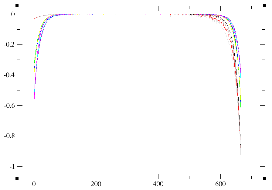
Here is the plot. How do I find the dimension of Gtau?
The dimension of Gtau is the number of correlated orbitals. You can deduce it from the number of columns in the Gtau file.
Looking at these plots, it seems like some of the curves are very noisy. The Green’s function should be convexe and non-convexity can lead to non-physical results. However, I would have thought that it should still work.
I need to know your parameters to provide help. What is your number of Monte Carlo cycles, thermalization, legendre coefficients? Also what is tsmear here?
You can do a calculation with a large tsmear for the non-interacting case. tsmear is a kind of temperature that by being increased will make the calculation easier and will not affect the non-interacting case (U=J=0). It should give better results. Look at how the calculated moment in OmegaMaxEnt change.
Many thanks for the info.
I have 10 columns and I guess it is from total 10 3d orbitals (spin up and down).
I set to tsmear = 0.025 eV
I set the number of cycle to higher value 3.d9 for MC, also thermalization to 100000.
However, I tried with smaller steps, tolvrs=1.d-4 and single iteration using smaller U=1 eV and J=0.2 eV. It seems the calculation converged after 7th cycle but, OmegaMaxEnt fails again. I tried with fitting polynomial order FNfitTauW=5 but still no success.
Here is the DMFT parameters:
usedmft1 0
usedmft2 1
dmftbandi 101
dmftbandf 110
dmft_solv 5 # QTQMC solver
dmftqmc_l 500 # Number of time slices for G(tau).
dmftqmc_n 3.d9 # Number of QMC sweeps
dmftqmc_therm 100000 # Thermalization
dmft_iter 1
dmft_nwli 100000
dmft_nwlo 1000
dmft_rslf 1
dmft_mxsf 0.7
dmft_dc 1
dmftctqmc_gmove 0
dmftctqmc_order 50
dmftcheck 0
DFT+U
usepawu1 1
usepawu 10
dmatpuopt 1
lpawu -1 2 -1 -1
upawu1 0.0 0.0 0.0 0.0 eV
jpawu1 0.0 0.0 0.0 0.0 eV
upawu2 0.0 0.733 0.0 0.0 eV
jpawu2 0.0 0.233 0.0 0.0 eV
Thanks!
PS: I tried with playing JH (0.2, 0.3, 0.4 eV etc.) keeping U fixed, sometimes it works sometimes not.
I’m not sure what to do. These are reasonable numbers and your curves are not that noisy, but still maybe too much.
A fifth order polynomial won’t be too good. Better would be a set of Legendre polynomials as in this paper. If you look at the coefficients of the polynomials, you should see them exponentially decay, until they reach noise. You can then truncated the series and that acts as noise filtering.
Other than that, I would try working at higher temperature, with less QMC cycles. There is should work pretty well. Then I would reduce temperature and see how increasing the number of cycles can help. But in principle you shouldn’t need this, as your curves are not that noisy to me. Perhaps Legendre filtering can solve your problem.
What does @amadon think?
Dear Olivier,
I was using dmft_solv = 5. In order to use Legendre polynomial, I have to use dmft_solv =6 or 7 using TRIQS library. Unfortunately, abinit was compiled without TRIQS library in m system. I will try that once I have it. However, suggestion to increase tsmear seemingly working keeping same QMC cycle.  Also, the Gtau plot looks good.
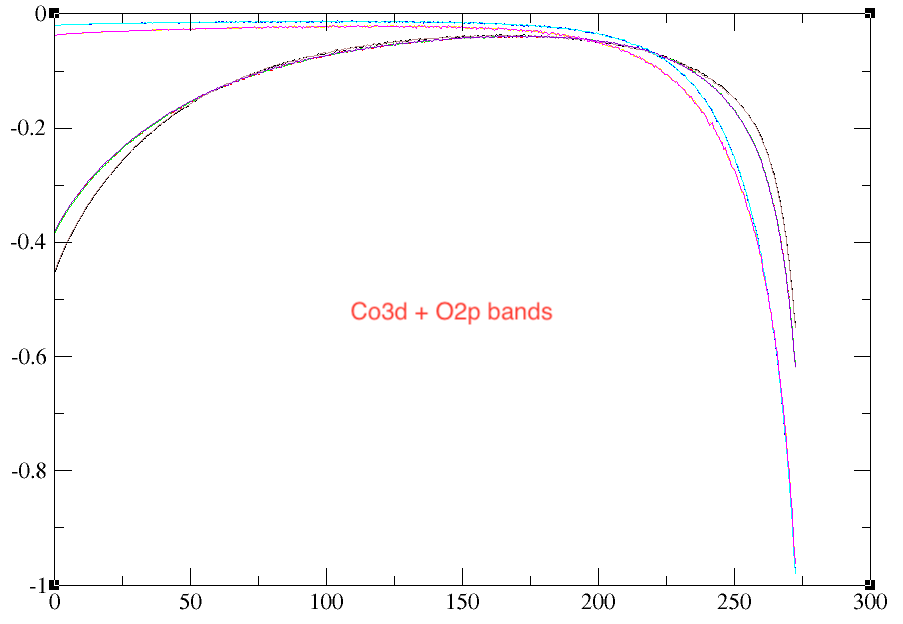
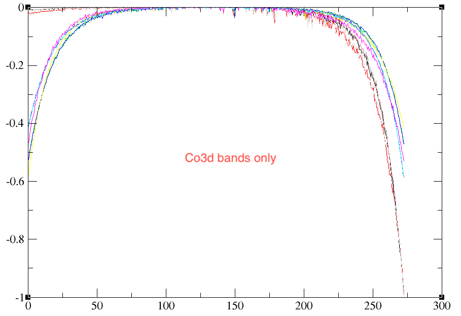
However, There is a problem when I consider different range of bands (dmftbandi and dmftbandf).
Top figure includes bands from Co3d and O2p whereas below figure consider only Co3d bands. All other calculation parameters were the same. The below figure gives more noisy results!
Could you please guide me in this regard, what could possibly give such noise?
Thanks!
R
So you should be careful with tsmear, since it changes the temperature of your calculation. It’s just a cheap way to do the calculation in less time, but if you still want to go to lower temperature, you need to change the number of time slices, frequencies, cycles and thermalization.
As for Legendre, you can use TRIQS, but you can also simply take your data and apply Legendre fitting to them, to filter the noise. I meant to do it independently from TRIQS.
As for the d-model (Co3d) vs dp-model (Co3d+O2p), they represent different systems in the end and will lead to slightly different results. You should know that the U and J is quite different between the two calculation. Indeed, in the Co3d model, oxygen electrons increase the screening of the Coulomb repulsion. Typically, in dp-model, you have Us~10eV for 3d electrons, while in d-model, you have Us~2-3eV. So in some sense, your dp-model is weakly interacting while your d-model is much more strongly interacting. What U/J have you used?
Best,
Olivier
Dear Olivier,
Thanks for your valuable advices and hints. As you mentioned in the last paragraph, this could be the problem since I used the same U=3eV and J=0.4 for both model! Therefore, I will check with U=1eV for the d-model as the dp model with U=3eV seemingly nicer, at least from green function plot.
Thanks and regards,
R